Problem

Let’s imagine a 2D problem. We have a set of points forming a unit circle whose radius is $r=1.0$. We have another set of points forming a square on the same 2D plane and its siDe length is $l=2.0$. Both the circle and the square center at the origin. Clearly we will not be able to find a linear map transforming the circle to a square. But if we try to find the “best” linear map to approximate the square, what shape will we get? Where in the math we introduce the approximation?

Analysis

I created a set of 2D points forming the circle and another set forming the squares. Both data are represented by a $2 \times m$ matrix where $m$ is the number of points. For the circle, we denote the data matrix as $\textbf{X}$, while for the square, the matrix is $\textbf{X}’$. We want to find the best linear map $\textbf{A}$ such that: \begin{equation} \textbf{X}’ \approx \textbf{A} \textbf{X}. \end{equation}

We will be using SVD on $\textbf{X}$ so that $\textbf{X} = \textbf{U} \Sigma \textbf{V}’$. So then our best $\textbf{A}$ can be written as: \begin{equation} \textbf{A} = \textbf{X}’ \textbf{V} \Sigma^{-1} \textbf{U}’. \end{equation}

Now here is the thing that I did not have a clear understanding before: if we plug back this $\textbf{A}$ into the transformation, we will not recover $\textbf{X}’$ because $\textbf{V}\textbf{V}’ \neq \textbf{I}$. I didn’t realize the fact that while $\textbf{V}’ \textbf{V} = \textbf{I}$, switching the order of the multipication will not give the same result. The columns of $\textbf{V}$ are orthonormal, but the rows aren’t. So what we get is in fact: \begin{equation} \textbf{X}’ \approx \textbf{X}’ \textbf{V} \textbf{V}’. \end{equation} The left hand side is what we want to get (the square), while the right hand side is the best we can achieve by a linear transformation from a circle.

I am still having a hard time ‘seeing’ the geometry behind the right hand side of above equation. One thing is clear, each transformed point can be expressed as: \begin{equation} \vec{y}_i = \sum_j <\vec{v}_i \vec{v}_j> \vec{x}’_j. \end{equation} Here $\vec{y}_i$ is a point that the best approximation a point on the square $\vec{x}’_i$. We can see it is obtained by some kind of average across all the points on the square. $\vec{v}_i$ is the normalized coordinates of the points on the circle in the new basis of $\textbf{U}$.

Plots

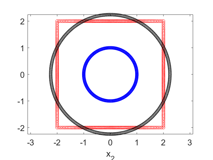
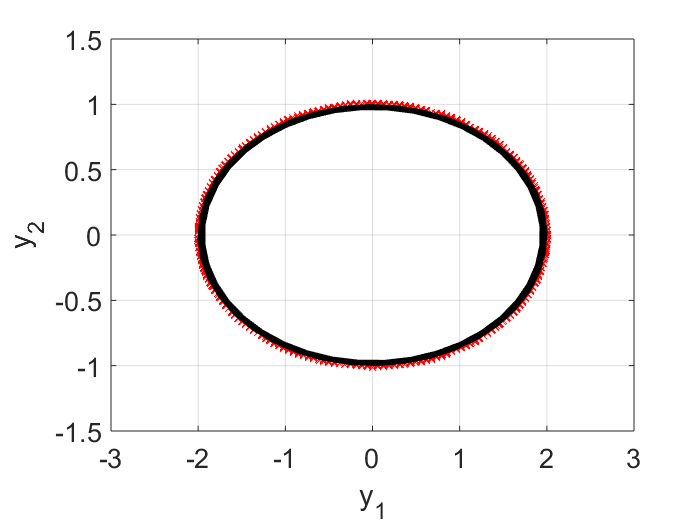
In the plot below, the blue dots are the circle points, the red are the square points. The black dots are the results of applying the best linear transform on the blue that tries to match with the red. No surprise it is another circle. This transformed circle can be created by either $\textbf{X}’ \textbf{V} \Sigma^{-1} \textbf{U}’ \textbf{X}$, or simply $\textbf{X}’ \textbf{V} \textbf{V}’$.

Data Creation

A 2D dynamical system

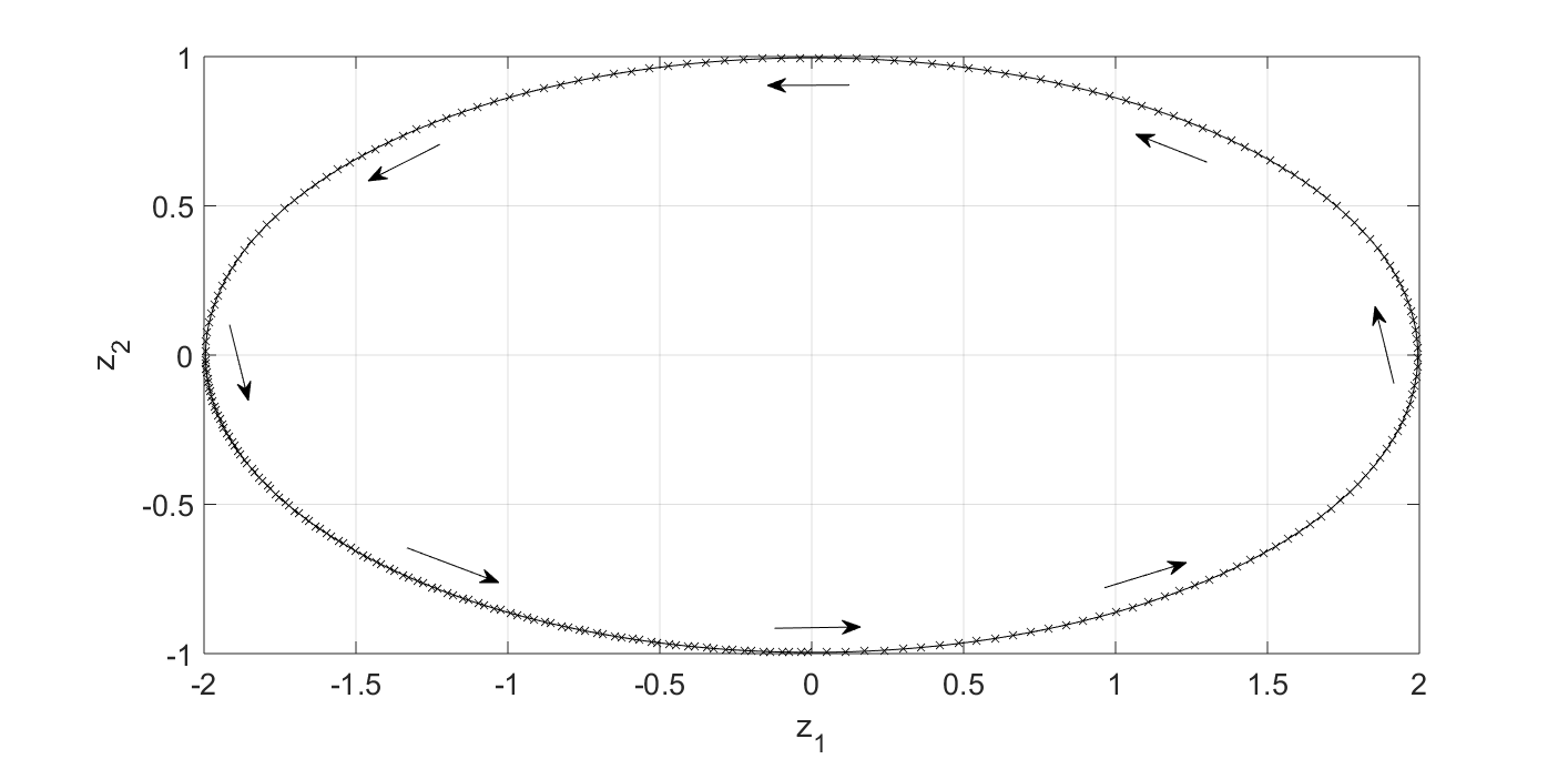
This first session has nothing to do with the DMD algorithm. The goal is to generate input data. Along the way, I will also try to refresh my memory on how to understand complex-value eigenvectors and eigenvalues for a linear dynamical system, which will help understand the DMD outputs later. Consider the following 2D dynamical system: \begin{equation} \frac{d z_1}{dt} = - 4 \pi z_2, \end{equation} \begin{equation} \frac{d z_2}{dt} = \pi z_1. \end{equation} We will use initial conditions $z_1(0)=2$ and $z_2(0)=0$. The solution to this linear dynamical system is $z_1(t)=2\cos(2\pi t)$ and $z_2(t) = \sin(2\pi t)$. It is a periodic solution with period $T=1.0$ second.

Detour: The eigen problem

Before generating data for the DMD algorithm, let’s first think about the eigenvectors and eigenvalues for this simple system. This will help understand the DMD algorithm later. If not interested in the detailed math, please skip this session and jump directly to the next session for input data generation.

Looking at Fig.1, it is clear that there should be no real-value eigenvector-eigenvalue pair for this system. Because if there is such a pair (and let’s denote it as $\vec{v}_z - \lambda_z$), it will satisfy: \begin{equation} \frac{d\vec{v}_z}{dt} = \textbf{A}_z \vec{v}_z = \lambda_z \vec{v}_z. \end{equation} Geometrically, the above equation says the flow direction $d\vec{v}_z$ is parallel to the state vector $\vec{v}_z$. We know we don’t have such a state because the flow in Fig.1 never points at the origin $z_1 = z_2 = 0$. So we know an eigen calculation will end up with complex-value results.

How should we understand the complex-value eigen results? Let’s say we have an eigenvector $\vec{v}_z = \vec{v}_r + i \vec{v}_i$ and an associated eigenvalue $\lambda_z = \lambda_r + i \lambda_i$. They will satisfy: \begin{equation} \frac{d\vec{v}_z}{dt} = \textbf{A}_z \left( \vec{v}_r + i \vec{v}_i \right) = \left(\lambda_r + i \lambda_i\right) \cdot \left( \vec{v}_r + i \vec{v}_i \right). \end{equation} Separating the real and imaginary parts, we have: \begin{equation} \textbf{A}_z \vec{v}_r = \lambda_r \vec{v}_r - \lambda_i \vec{v}_i, \end{equation} and \begin{equation} \textbf{A}_z \vec{v}_i = \lambda_r \vec{v}_i + \lambda_i \vec{v}_r. \end{equation} If $\lambda_r=0$, we will get: \begin{equation} \textbf{A}_z \vec{v}_r = - \lambda_i \vec{v}_i, \end{equation} and \begin{equation} \textbf{A}_z \vec{v}_i = \lambda_i \vec{v}_r. \end{equation} Geometrically, it says when the state is along $\vec{v}_r$, the flow should point along $\vec{v}_i$, and vice versa. This is exactly what Fig. 1 shows us. For example, at any point along the $z_1$ axis, the flow points at the $z_2$ direction. It’s also clear from the equation that $\lambda_r$ tells us whether the dynamics is winding out ($\lambda_r>1$), converging ($\lambda_r<1$) or following the same orbit again and again ($\lambda_r=1$), while $2\pi/\lambda_i$ gives us the period of the oscillation.

With the above knowledge, it is not surprising that when we perform eigen calculation for our system, we get $\vec{v}_r = [0.8944,0]’$, $\vec{v}_i = [0, -0.4472]’$, $\lambda_r = 0.0$ and $\lambda_i = 2\pi$.

How do we represent the solution (which is real value) using the eigen calculation results when we have complex eigenvectors and eigen values? Let’s first make a coordinate transform: \begin{equation} \vec{z} = \textbf{W} \vec{v}. \end{equation} Here $\textbf{W}$ is the eigenvector matrix. Note that this matrix needs not be orthonormal because there is no guarantee that $\textbf{A}_z$ is symmetric. In fact, for our problem, $\textbf{W} \textbf{W}’ = \text{diag}\left([1.6, 0.4]\right) \neq \textbf{I}$ (Here $\textbf{W}’$ is the complex conjugate transpose and \textbf{I} is the identity matrix). So when we revert the relation, we cannot use the transpose but have to do an inversion: \begin{equation} \vec{v} = \textbf{W}^{-1} \vec{z}. \end{equation}

The transformed $\vec{v}$ should satisfy: \begin{equation} \frac{d\vec{v}}{dt} = \left[\textbf{W}^{-1} \textbf{A}_z \textbf{W} \right] \vec{v} = \left[\textbf{W}^{-1} \Lambda \textbf{W} \right] \vec{v} = \Lambda \vec{v}. \end{equation}

So the solution to $\vec{v}$ is: \begin{equation} \vec{v}(t) = \exp \left(\Lambda t\right) \vec{v}(0). \end{equation} Here $\exp \left(\Lambda t\right)$ is a diagonal matrix with non-zero elements $\exp (\lambda_i t)$. Convert the solution back to $\vec{z}$, we can now express $\vec{z}(t)$ as: \begin{equation} \vec{z}(t) = \left[ \textbf{W} \exp \left(\Lambda t\right) \textbf{W}^{-1} \right] \vec{z}(0). \end{equation}

Input data generation

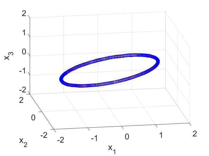
To generate input data for the DMD algorithm, I first generated snapshots of $\vec{z}(t)$ at different time and put them into a $2 \times m$ matrix, where $m$ is the number of snapshots. I then rotated the coordinate system by $45$ degrees on the 2D plane and generated snapshots of the same trajectory expressed in the new frame (which I call $\vec{y}$). In this new frame, the trajectory is just a $45$ degree tilted ellipse and it is stored in another $2 \times m$ matrix. To embed this 2D trajectory into a 3D space, I simply added a 3rd coordinate and make it $0.0$ for each point. This resulted in a $3 \times m$ matrix. Lastly I corrupted the 3D coordinates with noise and obtain the first $3 \times m$ input matrix $\textbf{X}$ for the DMD algorithm (Fig. 2).

The second input matrix is also of the size of $3 \times m$. Each column corresponds to the same column in $\textbf{X}$ but has a $\Delta t$ time shift. So if the first column in $\textbf{X}$ represents the state of the system at $t=0$ sec, then the first column in $\textbf{X}’$ represents the state at $t=0+\Delta t$ sec. With these two matrices, we can now explore the DMD algorithm.

The MATLAB code to generate these two input matrix is copied below.

  
%% Create input data for the DMD algorithm
% First create snapshots of z
t = 0:0.005:5;
z1 = 2.0 * cos(2.0*pi*t);
z2 = 1.0 * sin(2.0*pi*t);
Z = [z1; z2];
%plot(z1,z2); hold on;

% Then rotate the coordinate system to get a tilted ellipse
W = [sqrt(2.0)/2.0, -sqrt(2.0)/2.0; sqrt(2.0)/2.0, sqrt(2.0)/2.0];
Y = W*Z;
y1 = Y(1,:);
y2 = Y(2,:);
%plot(y1,y2); hold on;

% Embed the 2D ellipse into a 3D space, add noise
X = [Y; zeros(1,length(y1))];
x1 = X(1,:) + normrnd(0.0,0.01, 1,length(y1));
x2 = X(2,:) + normrnd(0.0,0.01, 1,length(y1));
x3 = X(3,:) + normrnd(0.0,0.01, 1,length(y1));
X = [x1;x2;x3];
%figure; plot3(x1,x2,x3); hold on; axis equal; grid on;

X(1,:) = movmean(X(1,:),5);
X(2,:) = movmean(X(2,:),5);
X(3,:) = movmean(X(3,:),5);

% Prepare the two DMD input matrics
xIndex=1:1:length(x1)-1;
Xp = X(:,xIndex+1);
X = X(:,xIndex);
  

Step 1 of DMD: Find the Reduced Order Space

In this session, we will use Single Value Decomposition (SVD) to find a reduced order space for the noisy 3D signal: \begin{equation} \textbf{X} = \textbf{U} \Sigma \textbf{V}^* \end{equation} Here the column vectors of the matrix $\textbf{U}$ are the new basis vectors, ranked such that the elements $\Sigma_{ii}$ in the diagonal matrix $\Sigma$ are in descending order. $\textbf{V}^*$ is the complex conjugate inverse of $\textbf{V}$. In this exercise the reduced order $r=2$ is assumed to be known so we only take the first two columns from $\textbf{U}$. Ref. 1 gives a procedure to determine the optimal reduced order for general problems. I want to focus on the DMD algorithm here so will take a shortcut to assume that $r=2$ is known.

The MATLAB code below calculates $\textbf{U}$, $\Sigma$ and $\textbf{V}$ from the input matrix $\textbf{X}$.

  
    [U, Sigma, V] = svd(X,'econ');
    r = 2;
    Ur = U(:,1:r);
    Sigmar = Sigma(1:r,1:r);
    Vr = V(:,1:r);
  

Note here the reduced order subspace is determined by $\textbf{X}$ and has nothing to do with the other input matrix $\textbf{X}’$. If you check the matrix $\textbf{Ur}$, you will find SVD correctly gets the reduced state space for us. On my computer (will be different for different random noise), the $3 \times 2$ $\textbf{Ur}$ matrix is:

  
    Ur = [-0.7075, 0.7067; -0.7067, -0.7075; -0.0002, -0.0001];
  

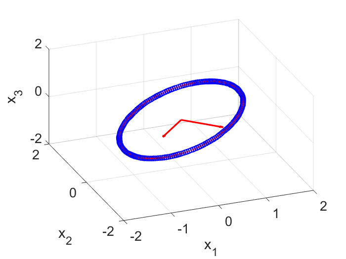
So the two axes are $\pm 45$ degrees on the $x_1$ and $x_2$ plane (Fig. 3). Next we will need to learn the dynamics from data in the reduced space spanned by these two vectors.

Step 2 of DMD: Find the Dynamics in the Reduced Order Space

We will use SVD to learn the 2D dynamics in the reduced space. In this step, the input matrix $\textbf{X}’$ will be used.

  
  Atilde = Ur'*Xp*Vr/Sigmar;
  

Here $\tilde{A}$ represents the learnt linear dynamics in the reduced order space, i.e., we learn from the input data that the evolution in the $y$ space is best approximated by $\vec{y}_{i+1} = \tilde{A} \vec{y}_i$. To check the quality of the learning, in the plot below, the raw input data points, projected on the $y$ space, are shown as dots, and the learnt dynamics is shown in a black curve. I can see on the first period, the learnt dynamics matches with the data quite well. But due to numeric error, i.e., $\text{det}(\tilde{A})$ is slightly less than $1.0$, in subsequent periodes, our trajectory begins to shrink (the black curve is spiraling inward). For real-life problems, this may not be an issue because most likely we will have some damping and so the real part of the eigen values won’t be exactly $1.0$.

Step 3 of DMD: Analytic Prediction of the Dynamics

Now we will do the eigen calculation on the learnt $\tilde{A}$.

  
  [West, Lambda] = eig(Atilde);
  

In the eigen space, the predicted 2D dynamics is: \begin{equation} \vec{z}(i) = \Lambda^i \vec{z}(0). \end{equation} Written in continuous time: \begin{equation} \vec{z}(t) = \exp \left[ \left(\log (\Lambda)/ \Delta t\right) t \right] \vec{z}(0) \end{equation}

The dynamics for $\vec{y}$ is: \begin{equation} \vec{y}(t) = \left[ \textbf{W} \exp \left[ \left(\log (\Lambda)/ \Delta t\right) t \right] \textbf{W}^{-1} \right] \vec{y}(0) \end{equation}

The dynamics for $\vec{x}$ is: \begin{equation} \vec{x}(t) = \left[ \textbf{U}_r \textbf{W} \exp \left[ \left(\log (\Lambda)/ \Delta t\right) t \right] \textbf{W}^{-1} \textbf{U}_r’ \right] \vec{x}(0) \end{equation}

The MATLAB code for the dynamics prediction is shown below.

  
predX = [];
for time=0:0.01:5
    predX = [predX, real(Ur*West*diag(exp(time*log(diag(Lambda))/0.005)) * inv(West) * Ur' * X(:,1))];
end
figure(h1);
plot3(predX(1,:),predX(2,:),predX(3,:),'g-','LineWidth',2.0); hold on;
  

If you run the entire code, you will find we succesfully recover the underlying 2D dynamics from the noisy 3D data.

Conclusion

From a set of noisy 3D data (note the DMD algorithm knows nothing about the physics that generates the data), we used DMD above to obtain a reduced order model such that the dynamics can be predicted analytically using a simple formula: \begin{equation} \vec{x}(t) = \left[ \textbf{U}_r \textbf{W} \exp \left[ \left(\log (\Lambda)/ \Delta t\right) t \right] \textbf{W}^{-1} \textbf{U}_r’ \right] \vec{x}(0). \end{equation}

For this example, the result looks trivial, but the DMD algorithm is impressive and is indeed a powerful tool for creating reduced-order models from data (say those obtained from high-fidelity models).

Reference

1.Brunton, S. L. & Kutz, J. N. Data-Driven Science and Engineering: Machine Learning, Dynamical Systems, and Control. (Cambridge University Press, 2019). doi:10.1017/9781108380690.

What DMD Does

DMD tries to learn a linear dynamical system from data and efficiently predict its behavior. Unlike training a deep learning neural network, however, DMD aims to do the “learning” efficiently. The data fed into the DMD algorithm are pairs of the state of a system separated by a small time interval $\Delta t$, for example, snapshots of the system at $t=10.0$s and $t=10.1$s. By digesting these pairs of “before and after” states, DMD learns how the system evolves in the time period of $\Delta t$. And if you know how a linear system changes in small $\Delta t$, you can predict its state at any time after an initial state is given. Note that here no physical law is used, we rely totally on data, although the data itself can be from some high-fidelity simulator that uses physics.

How DMD Works

Let’s first talk about the data fed into the DMD algorithm. Let $\vec{x}=[x_1, x_2, \cdots, x_n]^T$ be the state of a $n$-degrees-of-freedom dynamical system. Note that it is a column vector. We select a few, say $m$, snapshots of this system at different time and arrange these column vectors into a matrix $\textbf{X} = [\vec{x}(t_1), \vec{x}(t_2), \cdots, \vec{x}(t_m)]$. For each snapshot, we also get the state of the system after a time delay $\Delta t$, and arrange these states in a second matrix: $\textbf{X}’ = [\vec{x}(t_1+\Delta t), \vec{x}(t_2+\Delta t), \cdots, \vec{x}(t_m+\Delta t)]$. Now we would like to find a linear dynamical system such that: \begin{equation} \textbf{X}’ = \textbf{A} \textbf{X}. \end{equation} Here $\textbf{A}$ is a linear transformation that maps a column in $\textbf{X}$ to a corresponding column in $\textbf{X}’$.

Naturally, one would think that if we could do an “inverse” of the $n \times m$ matrix $\textbf{X}$ so that $\textbf{A} = \textbf{X}’ \textbf{X}^{-1}$, then our mission is accomplished. This is indeed a valid thought and SVD (singular value decomposition) can help us perform the psudo inverse. The problem is that when we have a large $n$, computing the $n \times n$ matrix $\textbf{A}$ becomes expensive, not to mention that later we may need to further compute some properties of the system by manipulating $\textbf{A}$ so we can efficiently predict the long-time evolution of the system. DMD gave us a procedure to find $\textbf{A}$ efficiently.

Since the main issue is that we have a high-dimension system with a large $n$, let’s imagine we have a magic solution to reduce the order of the system via a orthonormal mapping $\textbf{U}$: \begin{equation} \vec{x} = \textbf{U} \vec{y}. \end{equation} Here $\textbf{U}$ is a $n \times r$ matrix, and $\vec{y}$, our magic new reduced order state with less degrees of freedom, is a $r \times 1$ vector with $r < n$. Now the evolution of the system can be written as: \begin{equation} \textbf{U} \textbf{Y}’ = \textbf{A} \left( \textbf{U} \textbf{Y} \right). \end{equation} So the reduced order states follows: \begin{equation} \textbf{Y}’ = \left(\textbf{U}^* \textbf{A} \textbf{U} \right) \textbf{Y} = \textbf{A}_y \textbf{Y}. \end{equation} Here $\textbf{A}_y = \textbf{U}^* \textbf{A} \textbf{U}$ is a definition.

Assuming we know how to compute $\textbf{U}$ so we can convert our data from the $\vec{x}$ to the $\vec{y}$ space, then computing $\textbf{A}_y$ should be a “cheaper” operation. Since $\textbf{A}_y$ and $\textbf{A}$ are related, by learning $\textbf{A}_y$ from data, we also obtain $\textbf{A}$.

One benefit of obtaining a linear dynamical system is that we could “decouple” it into simpler forms to efficiently predict its long-time evolution. Decoupling the $n \times n$ $\textbf{A}$ matrix is expensive, but the lower order $\textbf{A}_y$ could help. As a classical eigen problem exercise, the next step is to find a tranform $\textbf{W}$ between $\vec{y}$ and a new state $\vec{z}$ (also of order $r$): \begin{equation} \vec{y} = \textbf{W} \vec{z}, \end{equation} so that the dynamics of $z_i$ are decoupled: \begin{equation} \textbf{Z}’ = \textbf{A}_z \textbf{Z}. \end{equation} Here $\textbf{A}_z = \text{diag}(\left[ \lambda_1, \lambda_2, \cdots, \lambda_r \right])$ is a $r \times r$ diagonal matrix. In the $z$ space, the decoupled variables evolve following: \begin{equation} z_i(t) = \exp \left(\lambda_i t \right) z_i(0). \end{equation} Here $i=1,2,\cdots,r$ and $\lambda_i$ are the complex-value eigen values.

To summarize, to reduce a high-dimensional data set to simple dynamics, one need to do two transforms, one from $\vec{x}$ to $\vec{y}$, followed by a second one from $\vec{y}$ to $\vec{z}$. Note that data matching is achieved when we compute $\textbf{A}_y$. Then we revert those transforms to predict how $\vec{x}$ will evolve.

The Unexplained Magic Step

I have left the “magic” step on transforming $\vec{x}$ to $\vec{y}$ unexplained above. This order reducing step can be achieved by using SVD decomposition of the $\textbf{X}$ matrix. It has been explained in the book (ref. 1) in earlier sessions.

Reference

1.Brunton, S. L. & Kutz, J. N. Data-Driven Science and Engineering: Machine Learning, Dynamical Systems, and Control. (Cambridge University Press, 2019). doi:10.1017/9781108380690.

What Transport Maps Can Do for Us

Imagine the following scenario. We know $x$ is a random variable that follows a standard Gaussian distribution. There is a complex function (maybe the function is only available numerically) $y=f(x)$ that transforms any given $x$ to a scalar $y$. What can we say about the distribution $P(y)$? Apparently one can sample a lot of $x$, pass them to the function $f$ to generate samples of $y$, then use statistics to describe the $y$ samples. This is great. But sometimes we may want to get an analytical expression for $P(y)$, or in some cases we are only given some samples of $y$ without any knowledge of $x$ and $f$ but we want to have a machinary to keep generating new samples of $y$ that minic the given samples. Transport maps can help.

Another scenario transport maps can help is when we are given an un-normalized distribution (maybe only numerically, i.e., if you give me a value $x$, I can tell you $P(x) \sim h(x)$ where $h$ doesn’t have an analytical expression but can be computed numerically following some procedure). Transport map can help us construct a normalized distribution and subsequently draw samples from it.

How Transport Maps Work

A transport map is a transform between a reference distribution and a targe distribution. We can use any simple distribution we like as our reference distribution and the target distribution is the one that we want to describe. The map is parametrized. The goal is to optimize those parameters so that after the transformation, the obtained target distribution matches any information we have about the target distribution. At the end of the day, finding a transport map becomes a loss minimization problem for parameter optimization.

Let’s say we are given some samples of $y$ and would like to (1) Obtain an analytic expression for $P(y)$ and (2) Generate more samples of $y$ ourselves. First thing we do is to pick a reference distribution we like. Say a standard normal distribution $P_x(x) \sim N(0,1)$. Then we define a parametrized map $y=f_\theta(x)$. Here $\theta$ are the parameters we will need to find/optimize later. Given any set of the parameters $\theta$, we can express $P_y(y)$ analytically as $P_y(y) = P_x({f_\theta}^{-1}(y)) | \nabla {f_\theta}^{-1} |$. Basically given any $y$, we say let’s transform it back to $x$ via $f_\theta^{-1}$ and see what’s the probability that $x$ appears ($P_x(x)$). We then adjust that with the Jacobian of the transform $f{_\theta}^{-1}$. With an parametrized and analytic $P_y(y)$, we now optimize the parameters so that $P_y(y)$ matches with the samples of $y$ given to us. This optimization can be done by minimizing the KL divergence between $P_y$ and the samples.

References

1.Marzouk, Y., Moselhy, T., Parno, M. & Spantini, A. An introduction to sampling via measure transport. arXiv:1602.05023 [math, stat] 1–41 (2016) doi:10.1007/978-3-319-11259-6_23-1.