Background

I had some confusion on SVD yesterday about when and where we introduce approximation on the DMD algorithm. My thought was that, intuitively, we cannot find an exact linear map to transform one set of points to another random set of points. Because of the randomness, the exact map most likely is nonlinear and nonlocal. But, in the 2nd step of DMD where we learn the linear dynamics from data, when and where do we make an approximation? This exercise was created to clear that confusion.

Problem

Let’s imagine a 2D problem. We have a set of points forming a unit circle whose radius is $r=1.0$. We have another set of points forming a square on the same 2D plane and its siDe length is $l=2.0$. Both the circle and the square center at the origin. Clearly we will not be able to find a linear map transforming the circle to a square. But if we try to find the “best” linear map to approximate the square, what shape will we get? Where in the math we introduce the approximation?

Analysis

I created a set of 2D points forming the circle and another set forming the squares. Both data are represented by a $2 \times m$ matrix where $m$ is the number of points. For the circle, we denote the data matrix as $\textbf{X}$, while for the square, the matrix is $\textbf{X}’$. We want to find the best linear map $\textbf{A}$ such that: \begin{equation} \textbf{X}’ \approx \textbf{A} \textbf{X}. \end{equation}

We will be using SVD on $\textbf{X}$ so that $\textbf{X} = \textbf{U} \Sigma \textbf{V}’$. So then our best $\textbf{A}$ can be written as: \begin{equation} \textbf{A} = \textbf{X}’ \textbf{V} \Sigma^{-1} \textbf{U}’. \end{equation}

Now here is the thing that I did not have a clear understanding before: if we plug back this $\textbf{A}$ into the transformation, we will not recover $\textbf{X}’$ because $\textbf{V}\textbf{V}’ \neq \textbf{I}$. I didn’t realize the fact that while $\textbf{V}’ \textbf{V} = \textbf{I}$, switching the order of the multipication will not give the same result. The columns of $\textbf{V}$ are orthonormal, but the rows aren’t. So what we get is in fact: \begin{equation} \textbf{X}’ \approx \textbf{X}’ \textbf{V} \textbf{V}’. \end{equation} The left hand side is what we want to get (the square), while the right hand side is the best we can achieve by a linear transformation from a circle.

I am still having a hard time ‘seeing’ the geometry behind the right hand side of above equation. One thing is clear, each transformed point can be expressed as: \begin{equation} \vec{y}_i = \sum_j <\vec{v}_i \vec{v}_j> \vec{x}’_j. \end{equation} Here $\vec{y}_i$ is a point that the best approximation a point on the square $\vec{x}’_i$. We can see it is obtained by some kind of average across all the points on the square. $\vec{v}_i$ is the normalized coordinates of the points on the circle in the new basis of $\textbf{U}$.

Plots

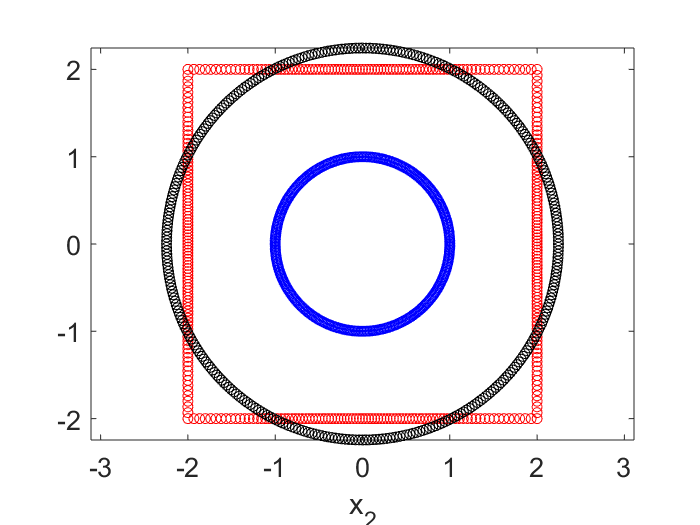
In the plot below, the blue dots are the circle points, the red are the square points. The black dots are the results of applying the best linear transform on the blue that tries to match with the red. No surprise it is another circle. This transformed circle can be created by either $\textbf{X}’ \textbf{V} \Sigma^{-1} \textbf{U}’ \textbf{X}$, or simply $\textbf{X}’ \textbf{V} \textbf{V}’$.