Problem Description

In this exercise, I would like apply the Dynamic Mode Decomposition (DMD) algorithm on a simple problem to familiarize myself with DMD. I will first generate the evolution history of a 2D oscillating system. I will then embed the 2D dynamics into a 3D space (put a planar curve into a 3D space) and corrupt the 3D signal with noise. The noisy 3D data will be fed into the DMD algorithm. I want to see if I can recover the true 2D dynamics from the corrupted 3D signal. The code below is written in MATLAB. I created the toy problem myself and modified the DMD codes in ref 1 to make it work for the problem.

Data Creation

A 2D dynamical system

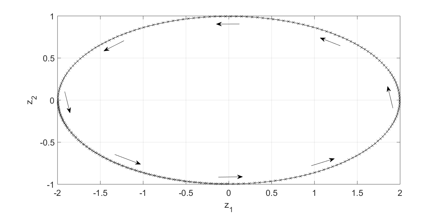
This first session has nothing to do with the DMD algorithm. The goal is to generate input data. Along the way, I will also try to refresh my memory on how to understand complex-value eigenvectors and eigenvalues for a linear dynamical system, which will help understand the DMD outputs later. Consider the following 2D dynamical system: \begin{equation} \frac{d z_1}{dt} = - 4 \pi z_2, \end{equation} \begin{equation} \frac{d z_2}{dt} = \pi z_1. \end{equation} We will use initial conditions $z_1(0)=2$ and $z_2(0)=0$. The solution to this linear dynamical system is $z_1(t)=2\cos(2\pi t)$ and $z_2(t) = \sin(2\pi t)$. It is a periodic solution with period $T=1.0$ second.

Detour: The eigen problem

Before generating data for the DMD algorithm, let’s first think about the eigenvectors and eigenvalues for this simple system. This will help understand the DMD algorithm later. If not interested in the detailed math, please skip this session and jump directly to the next session for input data generation.

Looking at Fig.1, it is clear that there should be no real-value eigenvector-eigenvalue pair for this system. Because if there is such a pair (and let’s denote it as $\vec{v}_z - \lambda_z$), it will satisfy: \begin{equation} \frac{d\vec{v}_z}{dt} = \textbf{A}_z \vec{v}_z = \lambda_z \vec{v}_z. \end{equation} Geometrically, the above equation says the flow direction $d\vec{v}_z$ is parallel to the state vector $\vec{v}_z$. We know we don’t have such a state because the flow in Fig.1 never points at the origin $z_1 = z_2 = 0$. So we know an eigen calculation will end up with complex-value results.

How should we understand the complex-value eigen results? Let’s say we have an eigenvector $\vec{v}_z = \vec{v}_r + i \vec{v}_i$ and an associated eigenvalue $\lambda_z = \lambda_r + i \lambda_i$. They will satisfy: \begin{equation} \frac{d\vec{v}_z}{dt} = \textbf{A}_z \left( \vec{v}_r + i \vec{v}_i \right) = \left(\lambda_r + i \lambda_i\right) \cdot \left( \vec{v}_r + i \vec{v}_i \right). \end{equation} Separating the real and imaginary parts, we have: \begin{equation} \textbf{A}_z \vec{v}_r = \lambda_r \vec{v}_r - \lambda_i \vec{v}_i, \end{equation} and \begin{equation} \textbf{A}_z \vec{v}_i = \lambda_r \vec{v}_i + \lambda_i \vec{v}_r. \end{equation} If $\lambda_r=0$, we will get: \begin{equation} \textbf{A}_z \vec{v}_r = - \lambda_i \vec{v}_i, \end{equation} and \begin{equation} \textbf{A}_z \vec{v}_i = \lambda_i \vec{v}_r. \end{equation} Geometrically, it says when the state is along $\vec{v}_r$, the flow should point along $\vec{v}_i$, and vice versa. This is exactly what Fig. 1 shows us. For example, at any point along the $z_1$ axis, the flow points at the $z_2$ direction. It’s also clear from the equation that $\lambda_r$ tells us whether the dynamics is winding out ($\lambda_r>1$), converging ($\lambda_r<1$) or following the same orbit again and again ($\lambda_r=1$), while $2\pi/\lambda_i$ gives us the period of the oscillation.

With the above knowledge, it is not surprising that when we perform eigen calculation for our system, we get $\vec{v}_r = [0.8944,0]’$, $\vec{v}_i = [0, -0.4472]’$, $\lambda_r = 0.0$ and $\lambda_i = 2\pi$.

How do we represent the solution (which is real value) using the eigen calculation results when we have complex eigenvectors and eigen values? Let’s first make a coordinate transform: \begin{equation} \vec{z} = \textbf{W} \vec{v}. \end{equation} Here $\textbf{W}$ is the eigenvector matrix. Note that this matrix needs not be orthonormal because there is no guarantee that $\textbf{A}_z$ is symmetric. In fact, for our problem, $\textbf{W} \textbf{W}’ = \text{diag}\left([1.6, 0.4]\right) \neq \textbf{I}$ (Here $\textbf{W}’$ is the complex conjugate transpose and \textbf{I} is the identity matrix). So when we revert the relation, we cannot use the transpose but have to do an inversion: \begin{equation} \vec{v} = \textbf{W}^{-1} \vec{z}. \end{equation}

The transformed $\vec{v}$ should satisfy: \begin{equation} \frac{d\vec{v}}{dt} = \left[\textbf{W}^{-1} \textbf{A}_z \textbf{W} \right] \vec{v} = \left[\textbf{W}^{-1} \Lambda \textbf{W} \right] \vec{v} = \Lambda \vec{v}. \end{equation}

So the solution to $\vec{v}$ is: \begin{equation} \vec{v}(t) = \exp \left(\Lambda t\right) \vec{v}(0). \end{equation} Here $\exp \left(\Lambda t\right)$ is a diagonal matrix with non-zero elements $\exp (\lambda_i t)$. Convert the solution back to $\vec{z}$, we can now express $\vec{z}(t)$ as: \begin{equation} \vec{z}(t) = \left[ \textbf{W} \exp \left(\Lambda t\right) \textbf{W}^{-1} \right] \vec{z}(0). \end{equation}

Input data generation

To generate input data for the DMD algorithm, I first generated snapshots of $\vec{z}(t)$ at different time and put them into a $2 \times m$ matrix, where $m$ is the number of snapshots. I then rotated the coordinate system by $45$ degrees on the 2D plane and generated snapshots of the same trajectory expressed in the new frame (which I call $\vec{y}$). In this new frame, the trajectory is just a $45$ degree tilted ellipse and it is stored in another $2 \times m$ matrix. To embed this 2D trajectory into a 3D space, I simply added a 3rd coordinate and make it $0.0$ for each point. This resulted in a $3 \times m$ matrix. Lastly I corrupted the 3D coordinates with noise and obtain the first $3 \times m$ input matrix $\textbf{X}$ for the DMD algorithm (Fig. 2).

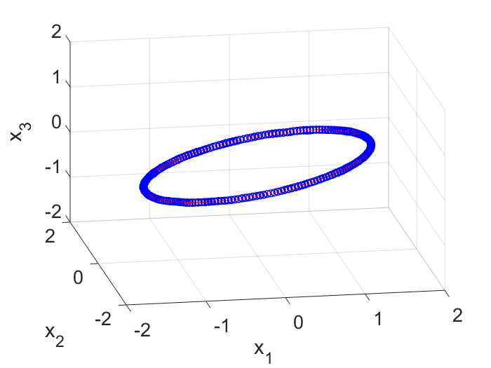
The second input matrix is also of the size of $3 \times m$. Each column corresponds to the same column in $\textbf{X}$ but has a $\Delta t$ time shift. So if the first column in $\textbf{X}$ represents the state of the system at $t=0$ sec, then the first column in $\textbf{X}’$ represents the state at $t=0+\Delta t$ sec. With these two matrices, we can now explore the DMD algorithm.

The MATLAB code to generate these two input matrix is copied below.

  
%% Create input data for the DMD algorithm
% First create snapshots of z
t = 0:0.005:5;
z1 = 2.0 * cos(2.0*pi*t);
z2 = 1.0 * sin(2.0*pi*t);
Z = [z1; z2];
%plot(z1,z2); hold on;

% Then rotate the coordinate system to get a tilted ellipse
W = [sqrt(2.0)/2.0, -sqrt(2.0)/2.0; sqrt(2.0)/2.0, sqrt(2.0)/2.0];
Y = W*Z;
y1 = Y(1,:);
y2 = Y(2,:);
%plot(y1,y2); hold on;

% Embed the 2D ellipse into a 3D space, add noise
X = [Y; zeros(1,length(y1))];
x1 = X(1,:) + normrnd(0.0,0.01, 1,length(y1));
x2 = X(2,:) + normrnd(0.0,0.01, 1,length(y1));
x3 = X(3,:) + normrnd(0.0,0.01, 1,length(y1));
X = [x1;x2;x3];
%figure; plot3(x1,x2,x3); hold on; axis equal; grid on;

X(1,:) = movmean(X(1,:),5);
X(2,:) = movmean(X(2,:),5);
X(3,:) = movmean(X(3,:),5);

% Prepare the two DMD input matrics
xIndex=1:1:length(x1)-1;
Xp = X(:,xIndex+1);
X = X(:,xIndex);
  

Step 1 of DMD: Find the Reduced Order Space

In this session, we will use Single Value Decomposition (SVD) to find a reduced order space for the noisy 3D signal: \begin{equation} \textbf{X} = \textbf{U} \Sigma \textbf{V}^* \end{equation} Here the column vectors of the matrix $\textbf{U}$ are the new basis vectors, ranked such that the elements $\Sigma_{ii}$ in the diagonal matrix $\Sigma$ are in descending order. $\textbf{V}^*$ is the complex conjugate inverse of $\textbf{V}$. In this exercise the reduced order $r=2$ is assumed to be known so we only take the first two columns from $\textbf{U}$. Ref. 1 gives a procedure to determine the optimal reduced order for general problems. I want to focus on the DMD algorithm here so will take a shortcut to assume that $r=2$ is known.

The MATLAB code below calculates $\textbf{U}$, $\Sigma$ and $\textbf{V}$ from the input matrix $\textbf{X}$.

  
    [U, Sigma, V] = svd(X,'econ');
    r = 2;
    Ur = U(:,1:r);
    Sigmar = Sigma(1:r,1:r);
    Vr = V(:,1:r);
  

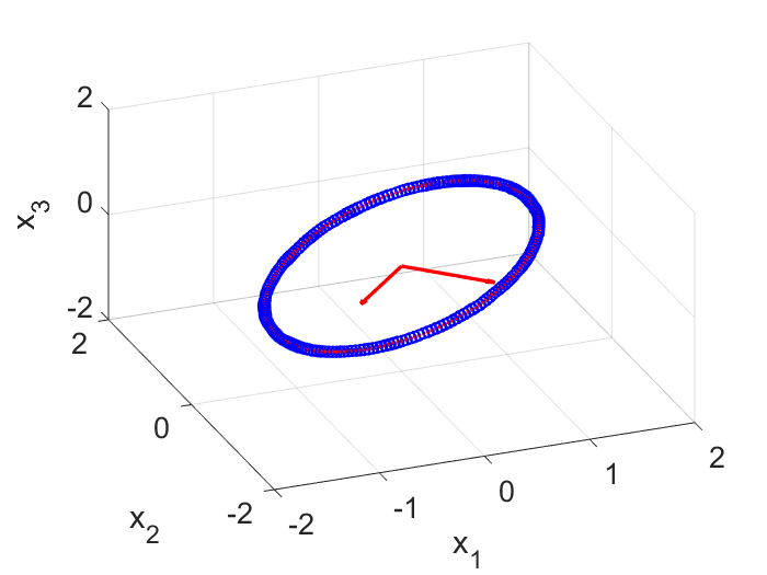
Note here the reduced order subspace is determined by $\textbf{X}$ and has nothing to do with the other input matrix $\textbf{X}’$. If you check the matrix $\textbf{Ur}$, you will find SVD correctly gets the reduced state space for us. On my computer (will be different for different random noise), the $3 \times 2$ $\textbf{Ur}$ matrix is:

  
    Ur = [-0.7075, 0.7067; -0.7067, -0.7075; -0.0002, -0.0001];
  

So the two axes are $\pm 45$ degrees on the $x_1$ and $x_2$ plane (Fig. 3). Next we will need to learn the dynamics from data in the reduced space spanned by these two vectors.

Step 2 of DMD: Find the Dynamics in the Reduced Order Space

We will use SVD to learn the 2D dynamics in the reduced space. In this step, the input matrix $\textbf{X}’$ will be used.

  
  Atilde = Ur'*Xp*Vr/Sigmar;
  

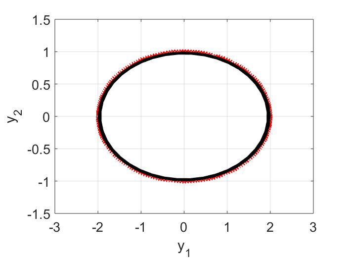
Here $\tilde{A}$ represents the learnt linear dynamics in the reduced order space, i.e., we learn from the input data that the evolution in the $y$ space is best approximated by $\vec{y}_{i+1} = \tilde{A} \vec{y}_i$. To check the quality of the learning, in the plot below, the raw input data points, projected on the $y$ space, are shown as dots, and the learnt dynamics is shown in a black curve. I can see on the first period, the learnt dynamics matches with the data quite well. But due to numeric error, i.e., $\text{det}(\tilde{A})$ is slightly less than $1.0$, in subsequent periodes, our trajectory begins to shrink (the black curve is spiraling inward). For real-life problems, this may not be an issue because most likely we will have some damping and so the real part of the eigen values won’t be exactly $1.0$.

Step 3 of DMD: Analytic Prediction of the Dynamics

Now we will do the eigen calculation on the learnt $\tilde{A}$.

  
  [West, Lambda] = eig(Atilde);
  

In the eigen space, the predicted 2D dynamics is: \begin{equation} \vec{z}(i) = \Lambda^i \vec{z}(0). \end{equation} Written in continuous time: \begin{equation} \vec{z}(t) = \exp \left[ \left(\log (\Lambda)/ \Delta t\right) t \right] \vec{z}(0) \end{equation}

The dynamics for $\vec{y}$ is: \begin{equation} \vec{y}(t) = \left[ \textbf{W} \exp \left[ \left(\log (\Lambda)/ \Delta t\right) t \right] \textbf{W}^{-1} \right] \vec{y}(0) \end{equation}

The dynamics for $\vec{x}$ is: \begin{equation} \vec{x}(t) = \left[ \textbf{U}_r \textbf{W} \exp \left[ \left(\log (\Lambda)/ \Delta t\right) t \right] \textbf{W}^{-1} \textbf{U}_r’ \right] \vec{x}(0) \end{equation}

The MATLAB code for the dynamics prediction is shown below.

  
predX = [];
for time=0:0.01:5
    predX = [predX, real(Ur*West*diag(exp(time*log(diag(Lambda))/0.005)) * inv(West) * Ur' * X(:,1))];
end
figure(h1);
plot3(predX(1,:),predX(2,:),predX(3,:),'g-','LineWidth',2.0); hold on;
  

If you run the entire code, you will find we succesfully recover the underlying 2D dynamics from the noisy 3D data.

Conclusion

From a set of noisy 3D data (note the DMD algorithm knows nothing about the physics that generates the data), we used DMD above to obtain a reduced order model such that the dynamics can be predicted analytically using a simple formula: \begin{equation} \vec{x}(t) = \left[ \textbf{U}_r \textbf{W} \exp \left[ \left(\log (\Lambda)/ \Delta t\right) t \right] \textbf{W}^{-1} \textbf{U}_r’ \right] \vec{x}(0). \end{equation}

For this example, the result looks trivial, but the DMD algorithm is impressive and is indeed a powerful tool for creating reduced-order models from data (say those obtained from high-fidelity models).

Reference

1.Brunton, S. L. & Kutz, J. N. Data-Driven Science and Engineering: Machine Learning, Dynamical Systems, and Control. (Cambridge University Press, 2019). doi:10.1017/9781108380690.